Article Text

Abstract
Background The potential impact fraction is a measure of effect that calculates the proportional change in disease risk after a change in the exposure of a related risk factor. Potential impact fractions are increasingly used to calculate attributable fractions when the lowest exposure is non-zero.
Methods Risk-factor exposure can be expressed as a categorical or a continuous variable. For a categorical risk factor, a change in risk-factor exposure can be expressed as a change in the proportion of the population in each category (‘proportions shift’). For a continuous risk factor, the change is expressed as a change in its parameters (‘distribution shift’). A third method (‘RR shift’) takes elements of both the categorical and the continuous approach. We compare the three calculation methods using hypothetical data on BMI and an intervention that affects the obese category.
Results The ‘proportion shift’ calculation produces non-linear artefacts and is best avoided. The ‘RR shift’ and ‘distribution shift’ calculation require the estimation of an RR function to describe excess risk, but perform much better.
Conclusion The ‘proportion shift’ calculation is best avoided. The ‘RR shift’ and ‘distribution shift’ calculation produce virtually the same results. For evaluating high-risk strategies, the ‘RR shift’ calculation is the simplest and therefore preferred. The ‘distribution shift’ is best suited for evaluating population strategies.
- Epidemiologic methods
- evaluation studies
- potential impact fraction
- computing eqs
Statistics from Altmetric.com
Background
The potential impact fraction (PIF) is an epidemiological measure of effect that calculates the proportional change in average disease incidence (or prevalence or mortality) after a change in the exposure of a related risk factor.1 In its simplest form, with just one category of exposed, the equation for the PIF is:
The PIF is closely related to a more widely used measure that goes by a number of different names such as ‘attributable fraction’ (AF), ‘population attributable fraction’ and ‘etiologic fraction,’ while these terms have also been used for differently defined measures. The AF we refer to is defined as:
From equation 1, it is easy to see that the AF is a special case of the PIF that calculates the proportional change in incidence when the risk-factor exposure (P*) would be reduced to zero. The interpretation then is that the change is the proportion of incidence that can be attributed to the related risk factor.3 In this role, the AF has been used to estimate risk-factor attributable burden of disease and costs.4
For many risk factors (such as BMI and blood pressure), however, a zero exposure is not an appropriate minimal exposure. Calculation of an attributable fraction then requires the definition of a non-zero lowest exposure, the so-called ‘theoretical minimum risk.’5 The AF then is calculated using current exposure, the theoretical minimum risk and the equation for the PIF.6 7 Because of this development, potential impact fractions have taken on a new importance.8
Risk-factor exposure is almost always a continuous phenomenon, but in practice epidemiologists have mostly been using categories. For example, the WHO categories for BMI are ‘normal’ (18.5≤BMI<25), ‘overweight’ (25≤BMI<30) and ‘obese’ (BMI≥30).9 In reality, BMI is much better described by a (log)normal distribution.10
Nevertheless, when evaluating effects of risk-factor exposure and interventions, we are mostly stuck with categories. For one thing, since epidemiologists have been using categories, their reported results (such as relative risks) are in categories, too. For another, many interventions are targeted at high-risk groups, in the case of BMI, for example, at the obese. At the same time, the effects of a population strategy, such as media campaigns, are best evaluated using a continuous description of risk-factor exposure.11
This paper examines the divide between categorical and continuous risk-factor exposure descriptions in the calculation of PIFs. We compare the results of calculating PIFs using risk-factor categories with those using a continuous risk-factor distribution. We introduce a third method that takes elements of both the categorical and the continuous approach. We use the example of BMI, with hypothetical but realistic data.
Methods
We distinguish between three methods of calculating PIFs. In the ‘proportions shift’ method, both risk-factor exposure and relative risks are categorical. In the ‘distribution shift’ method both the risk-factor exposure and the RR are described by continuous functions. With the ‘RR shift’ method the risk-factor exposure is categorical, but the RR is continuous, using a RR function.
Proportions shift
An intervention in a categorical risk factor can be described by a change in the proportion of the population per category. For a risk factor with n categories, the equation for the PIF then becomes12:
In this ‘proportions shift’ calculation, the main issue is to determine what the proportion in each category is after the intervention. For example, suppose that an intervention targeted at obese people makes them lose 2 kg. To determine how many would shift from the category ‘obese’ to ‘overweight,’ it is necessary to know what the distribution of BMI within the category ‘obese’ is, either from data of the population on the personal level or by assuming a distribution (in addition, an average height must be known or assumed).
Distribution shift
The second way to calculate the effect of the same intervention is to assume a continuous risk-factor distribution, and calculate the effect of the intervention on its parameters. For this ‘distribution shift’ calculation, the PIF equation is13:
RR shift
The same intervention can also be described by a change in the relative risks of the categories, while keeping the proportion in each category constant. For this ‘RR shift’ calculation, the equation for the PIF becomes:
The main issue now of course is to obtain the RRc*, given the intervention. This can be done by assuming a functional relationship between the level of risk-factor exposure and the RR. Assuming that the observed relative risks per category pertain to the mean risk level in that category allows us to estimate a functional relationship, such as a log-linear function. If a ‘per unit’ RR is available, this can be used directly. In both cases the mean risk level needs to be calculated in all categories, again either from observed data or by assuming an underlying continuous risk-factor distribution.
Risk-factor distributions and RR functions
We have implemented these methods for a hypothetical population with a mean BMI of 25 and an SD of 3. Both normal and log-normal distributions have been implemented. For the categorical calculation, we assumed an RR of 1.5 for overweight and 2 for obese, which corresponds with the risk of total mortality in adults in these categories.14
For the RR functions, we implemented two functions. First, a log-linear function:
Second, a ‘per unit’ function:
Two distributions and two RR functions give four combinations. For each combination we calculated the effect of interventions for the obese category ranging from 1 to 20 kg weight loss for each of the three PIF equations. Calculations are done in MS Excel, with the help of additional software to do the integration of equation 5. The spreadsheet and additional software (an Excel add-in) are available from http://www.epigear.com/.
Results
Table 1 shows the proportions in each BMI category, average BMI per category and relative risks from the RR functions, for both the normal and the log-normal BMI distributions. Differences between the two BMI distributions are small, with the log-normal having somewhat more people in the ‘normal’ and ‘obese’ categories. The ‘per unit’ RR function results in somewhat higher relative risks than the log-linear RR function, and there are also small differences between the results from the RR functions of each BMI distribution because of the differences in average BMI.
Risk-factor distributions and relative risk (RR) functions
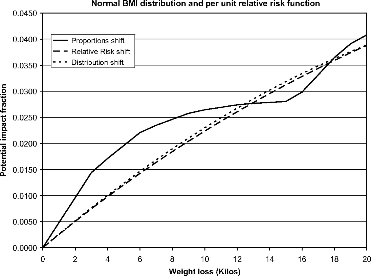
Figure 1 shows the results from the combination of a normal risk-factor distribution and a log-linear RR function. The ‘RR shift’ and ‘distribution shift’ calculations yield virtually undistinguishable results, and the ‘proportional shift’ calculation is highly non-linear, yielding at times higher and lower results.

Potential impact fractions as a function of intervention size in obese people, for three calculation methods, a normal BMI distribution and a log-linear relative risk function.
Figure 2 shows the results from the combination of a normal risk-factor distribution and a ‘per unit’ RR function. Again the ‘RR shift’ and ‘distribution shift’ calculations are virtually undistinguishable, and the ‘proportional shift’ calculation shows the same non-linear pattern as with the linear RR function.
Potential impact fractions as a function of intervention size in obese people, for three calculation methods, a normal BMI distribution and a ‘per unit’ relative risk function.
The results for the log-normal risk-factor distribution are very similar to the normal distribution (see supplementary material).
Conclusion
We performed a comparative assessment of three different calculation methods of PIFs. The PIF as presented in equation 1 is a linear function of the intervention size: with increasing size of the intervention, the PIF will linearly go to its maximum value that is given by the attributable (‘excess’) fraction of equation 3. When a non-linear RR function is used, the resulting PIF will become non-linear as well; however, for small ranges and low values of the PIF, as in the present calculations where the value ranges from 0 to well below 0.05, the relationship between intervention size and PIF is linear to a close approximation. This behaviour is displayed by the ‘RR shift’ and ‘distribution shift’ calculations that yield virtually the same results.
The ‘proportional shift’ calculation, on the other hand, introduces non-linearities where there should be none. At first, the ‘proportional shift’ calculation overestimates the effect because a small shift in weight earns a large shift in RR. As more of the obese group ends up in overweight, the ‘proportional shift’ calculation becomes progressively less sensitive to additional weight loss, until the loss becomes so large (at 16 kilos) that the first formerly obese end up in the ‘normal weight’ category, and the PIF takes off again.
These are clearly artefacts caused by the categorisation of the risk-factor distribution in combination with a categorical RR. When the number of categories increases, the episodes of over- and underestimation will become correspondingly more numerous but smaller; in the end, with a large number of categories, the ‘proportions shift’ will approximate the ‘distribution shift’ method.
The intervention that lowers the weight in the obese category results in a lower mean and SD of the normal and log-normal distributions. The actual BMI distribution becomes progressively less (log)normal with additional weight loss, but this is ignored by the ‘distribution shift’ calculation. It is in fact rather surprising that shifting the whole distribution produces such similar results as in the ‘RR shift’ calculation.
In conclusion, exposure categories in continuous risk factors are a nuisance but also a fact of life. For a continuous risk factor, the gold standard is to describe it by a continuous function. However, to evaluate interventions aimed at specific risk categories, there is no way to get around these.
Of the three ways to calculate the effect of interventions on a high-risk category presented here, the ‘proportional shift’ calculation, which redistributes people to a different category, is the most intuitive, was the one originally proposed1 and probably is the most used.15–17 However, it produces artefactual non-linearities and, depending on size of intervention, over- and underestimates. This calculation method is therefore best avoided.
Both the ‘RR shift’ and the ‘distribution shift’ calculation require the estimation of a RR function, but that seems a small price to pay for a vastly better performance. Of the two, the ‘RR shift’ calculation is the simplest, and will, given a valid RR function, produce correct results. With a software add-in, the ‘distribution shift’ calculation is also simple, but it ignores the departure from the assumed distribution. This calculation method is best suited to evaluate population instead of high-risk strategies.
What is already known on the subject
The potential impact fraction (PIF) is a measure of effect that calculates the proportional change in disease frequency, given a change in related risk-factor exposure.
Calculation methods for categorical (‘proportions shift’) and continuous (‘distribution shift’) risk-factor distributions exist.
What this study adds
We show that the ‘proportions shift’ calculation introduces artefactual non-linearities and, depending on amount of weight loss, either over- or underestimates the PIF.
We introduce a third calculation method (‘RR shift’) that combines elements of the categorical and continuous calculation methods, and avoids the problems of the ‘proportions shift’ method.
References
Footnotes
Funding National Health & Medical Research Council.
Competing interests None.
Provenance and peer review Not commissioned; externally peer reviewed.